Requires: Utmost IV, SmartSpice, SmartView
Minimum Versions: Utmost IV 1.11.2.R, SmartSpice 4.10.6.R, SmartView 2.28.2.R
This example describes how to perform a bipolar AC measurement and then plot the
ft and fmax characteristics.
The project file
acq_ex14.prj
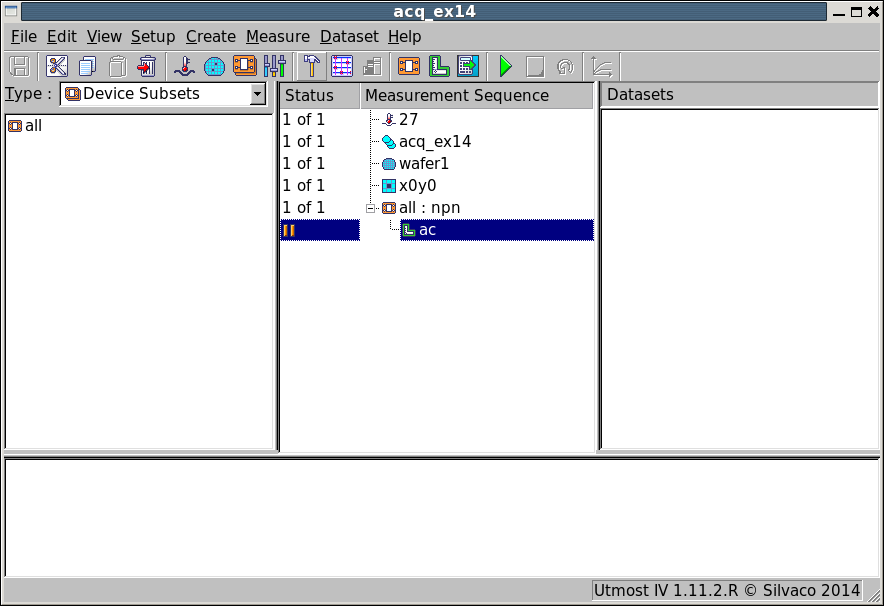
for this example should be loaded into your database. When opened, the
project will look as shown in
acq_ex14_01.png
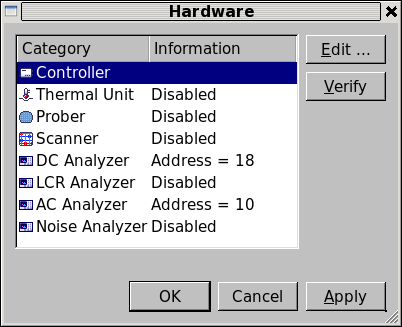
. In the project hardware, the DC Analyzer and AC Analyzer are enabled for measurement
as shown in
acq_ex14_02.png
.
AC measurements are typically performed using a network analyzer which measures
s-parameters at multiple frequencies. The analyzer has two ports which are connected
to the bipolar transistor. Port 1 is connected to the base and port 2 is connected to
the collector. The emitter of the transistor is connected to the common ground of the
two ports. During the AC measurement, the s-parameters or scatter parameters will be
measured between these two ports. These s-parameters are complex values, having both
real and imaginary parts. For a two port measurement, there will be four s-parameters
which are commonly known as s11, s12, s21 and s22.
Once you have the s-parameters of your two port system, you can convert these
into other more useful forms, such as impedances, admittances and gains. All of
these impedances, admittances and gains are also complex values. This is all
automatically done for you by Utmost IV. In addition, Utmost IV also provides useful
shortcuts for specifying the magnitude, phase, real and imaginary parts of these
complex numbers.
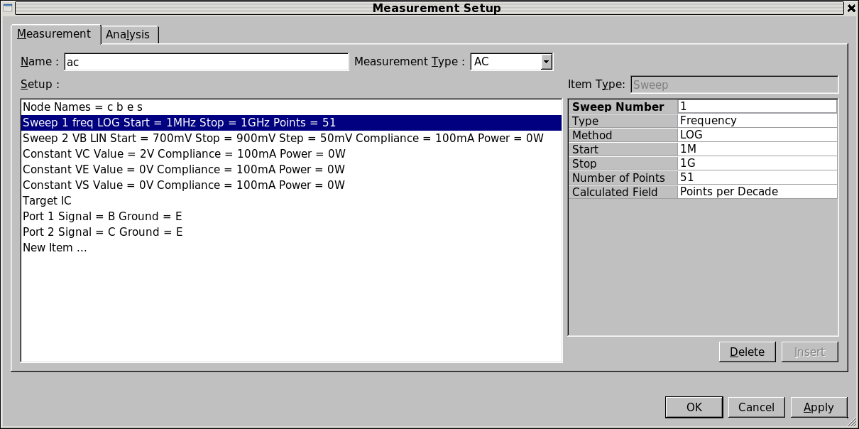
The project contains a single AC measurement setup which is defined as shown in
acq_ex14_03.png
. For all AC measurements, the frequencies
at which the s-parameters will be measured are defined by the first sweep in the
measurement setup. The measurement setup also defines one or more DC bias points at
which the frequency dependent s-parameters will be measured. In this example, the
collector voltage is fixed at 2 volts, while the base voltage is swept from 0.7 to
0.9 volts in 50mV steps. At each one of these DC bias points, the s-parameters will
be measured across the frequency range.
The exact frequency and bias range you need to use will be determined by
the device being measured and also by the limitations of your test equipment.
Unity Gain Bandwidth, ft
The unity gain bandwidth (ft) is defined as the frequency at which the forward
small signal current gain (hfe) of the transistor has a magnitude of 1. A magnitude
of 1 is equivalent to zero dB.
h21 = i2/i1 = ic/ib = hfe = forward current gain
h21m = magnitude of h21
20 * log10 (h21m) = magnitude of h21 in dB
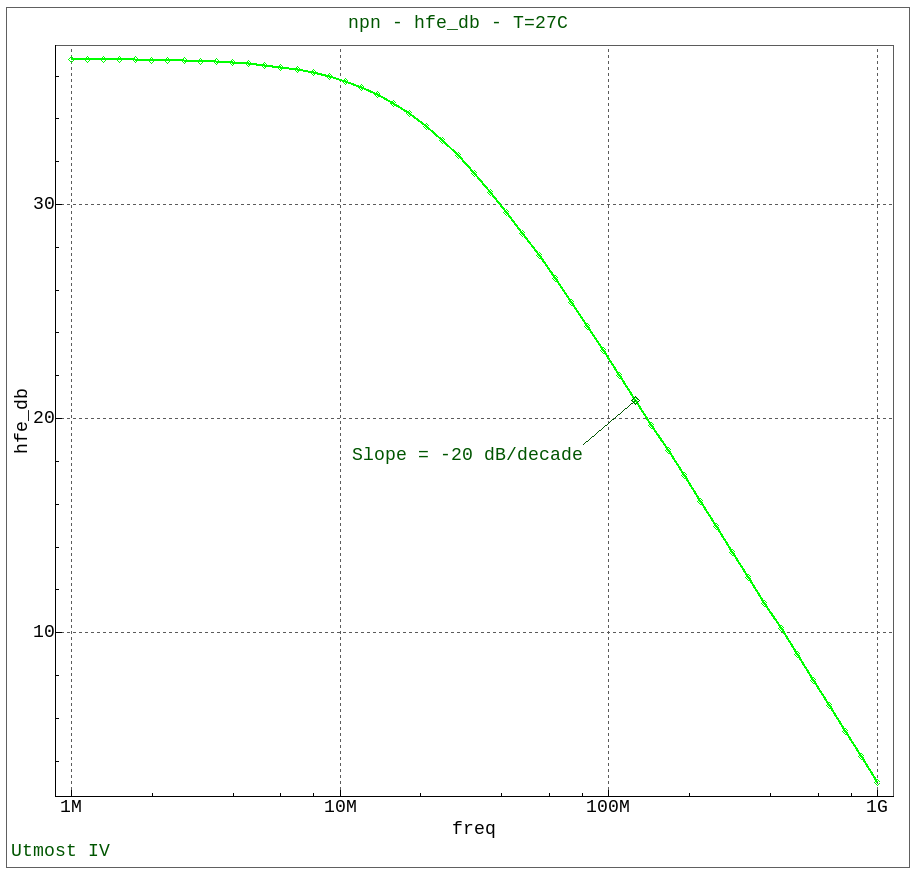
If you plot the magnitude of h21 in dB vs frequency on a log scale, you will
get a plot which looks like
acq_ex14_04.png
. At low frequency the gain of the bipolar transistor is constant. Once you
reach a certain frequency, the gain will reduce with a single pole roll off.
The slope of this reduction in gain will be -20dB/decade of frequency. The
frequency at which the gain is reduced to 0dB is the unity gain bandwidth or
ft for this specific DC bias point.
Utmost IV provides a special function which will extract the ft characteristic
for each DC bias point.
ft = ft (freq, h21m, 0, 0, 3, -20, 0)
The value of ft can then be plotted vs the DC bias conditions.
Maximum Oscillation Frequency, fmax
This is defined as the frequency at which the forward small signal power gain of
the transistor has a magnitude of 1. A magnitude of 1 is equivalent to zero dB.
The power gain of this two port system is best described using Mason’s invarient
unilateral power gain, U. [1][2]
U = pow(mag(z12-z21),2)/(4*(z11r*z22r-z12r*z21r))
10 * log10 (mag (U)) = magnitude of U in dB
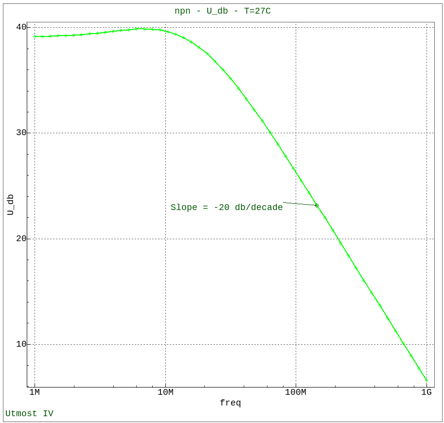
If you plot the magnitude of U in dB vs frequency on a log scale, you will
get a plot which looks like
acq_ex14_05.png
. At low frequency the gain of the bipolar transistor is relatively constant.
Once you reach a certain frequency, the gain will reduce with a single pole roll
off. The slope of this reduction in gain will be -20dB/decade of frequency. The
frequency at which the power gain is reduced to 0dB is the maximum oscillation
frequency or fmax for this specific DC bias point.
We can make use of the special ft function to extract fmax as well by remembering
the following.
10 * log 10 (x) = 20 * log10 (sqrt (x))
fmax = ft (freq, sqrt (U), 0, 0, 3, -20, 0)
The value of fmax can then be plotted vs the DC bias conditions.
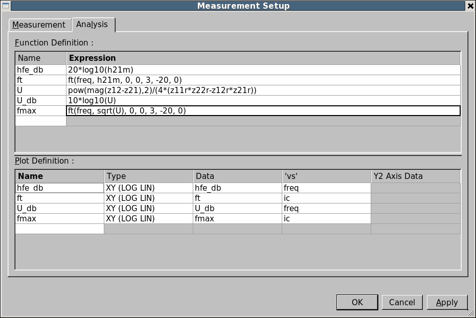
The analysis section of the measurement setup includes the function and plot
definitions to display the characteristic gain vs frequeny plots and also the
ft and fmax vs DC bias condition plots as shown in
acq_ex14_06.png
.
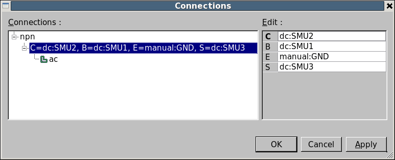
You must also define the DC instrument source connections. The measurement
connections are shown in
acq_ex14_07.png
. In this example, DC SMU1 is connected to Port 1 and to the base of the
bipolar, DC SMU2 is connected to Port 2 and to the collector of the bipolar.
The emitter is connected to the AC ground of the network analyzer. In this case,
we set the connection for this terminal to ‘manual ground’. Finally the substrate
of the transistor is biased using DC SMU3.
Before measuring the bipolar transistor it is essential that you calibrate the
AC network analyzer instrument and perform de-embedding on the test structures
that you have available. To begin the calibration and de-embedding process,
select
Measure->Calibrate
from the project menu.
Once calibration is done, AC measurement will be performed by selecting
Measure->Run
from the project menu.
For this example, we can now switch the project into its simulation mode by selecting
Measure->Simulation
from the project menu. This will allow us to view the typical characteristics which will
be generated when the measurement is performed.
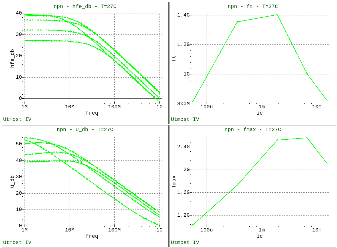
When the measurement sequence is run, the measured data will be automatically stored in
the database and the measured results will be shown in the dataset selector area of the
acquisition project as shown in
acq_ex14_08.png
.
These four plots show how the transistor small signal forward current and power gain vary
with frequency and DC bias conditions. The ft and fmax figures of merit are also calculated
and plotted. In this simulation example, the peak ft value is around 1.4 GHz and the
peak fmax value is around 2.5 GHz.
References:
[1] Mason, Samuel (June 1954). “Power Gain in Feedback Amplifiers”
IRE Transactions on Circuit Theory, Vol 1, no 2
[2] Gupta, Madhu (May 1992). “Power Gain in Feedback Amplifiers, a Classic Revisited”
IEEE Transactions on Microwave Theory and Techniques, Vol 40, no 5
Graphics