Requires: SmartSpice & Smartview

Minimum Versions: SMARTSPICE 4.30.5.R + SMARTVIEW 2.34.3.R

The SmartView application allows users to look at distributions of a regular occouring event. in this example we run a Monte-Carlo analysis on a 3 stage {textview} 3stage_inverter_monte.in Ring Oscillator to look at the frequency variation and plot a distribution of the frequency change and even fit a distribution curve to the histogram.

1. Source input deck netlist in SmartSpice application.

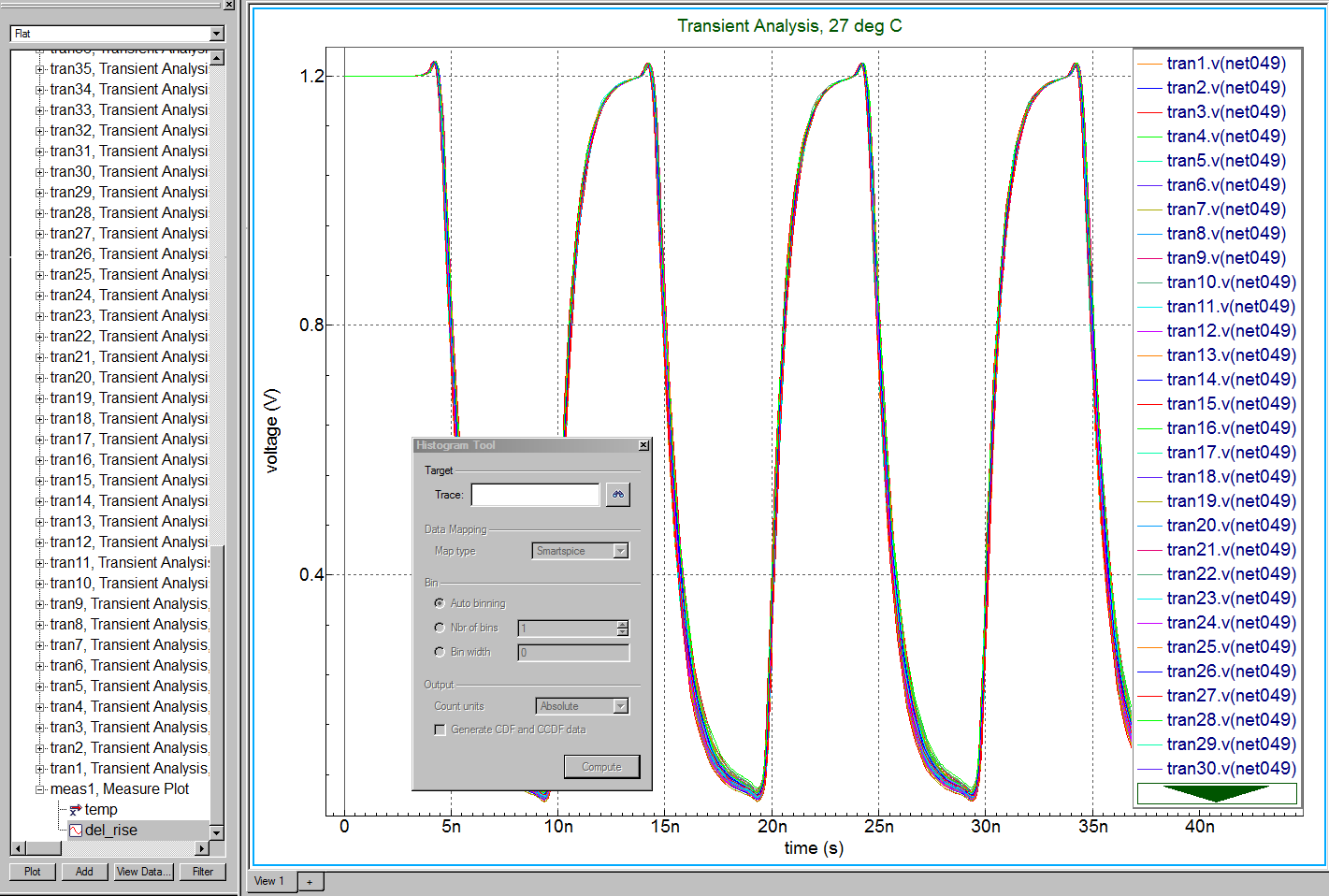
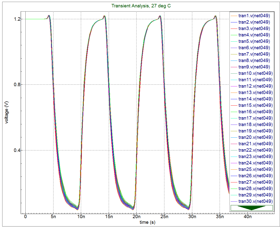
2. In the vectors window of SmartSpice select all the Tran1 to Tran100 plots in the upper half of the window and the vector(net049) in the lower “vector” window then hit plot button. You will then see a plot
like this in smartview.

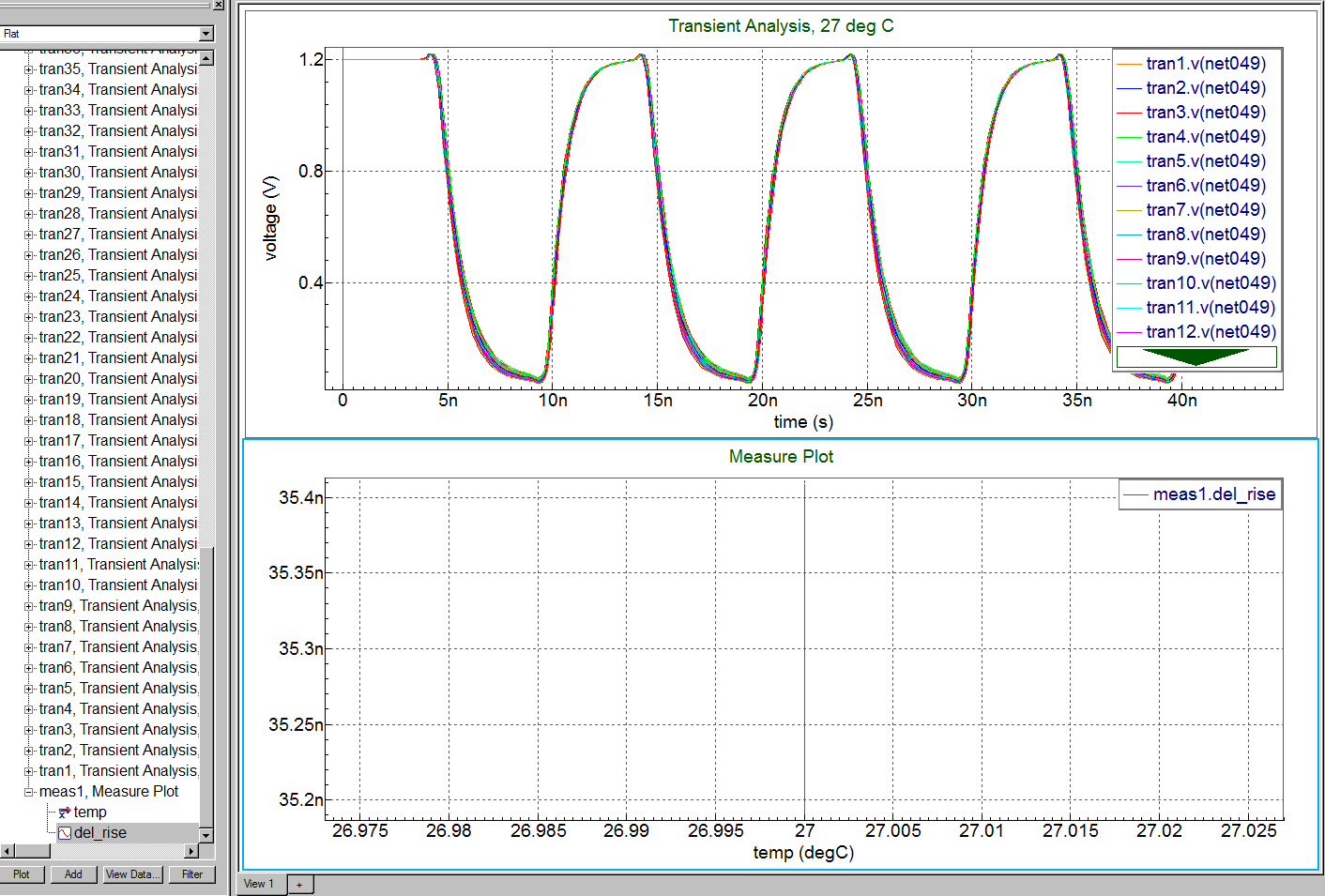
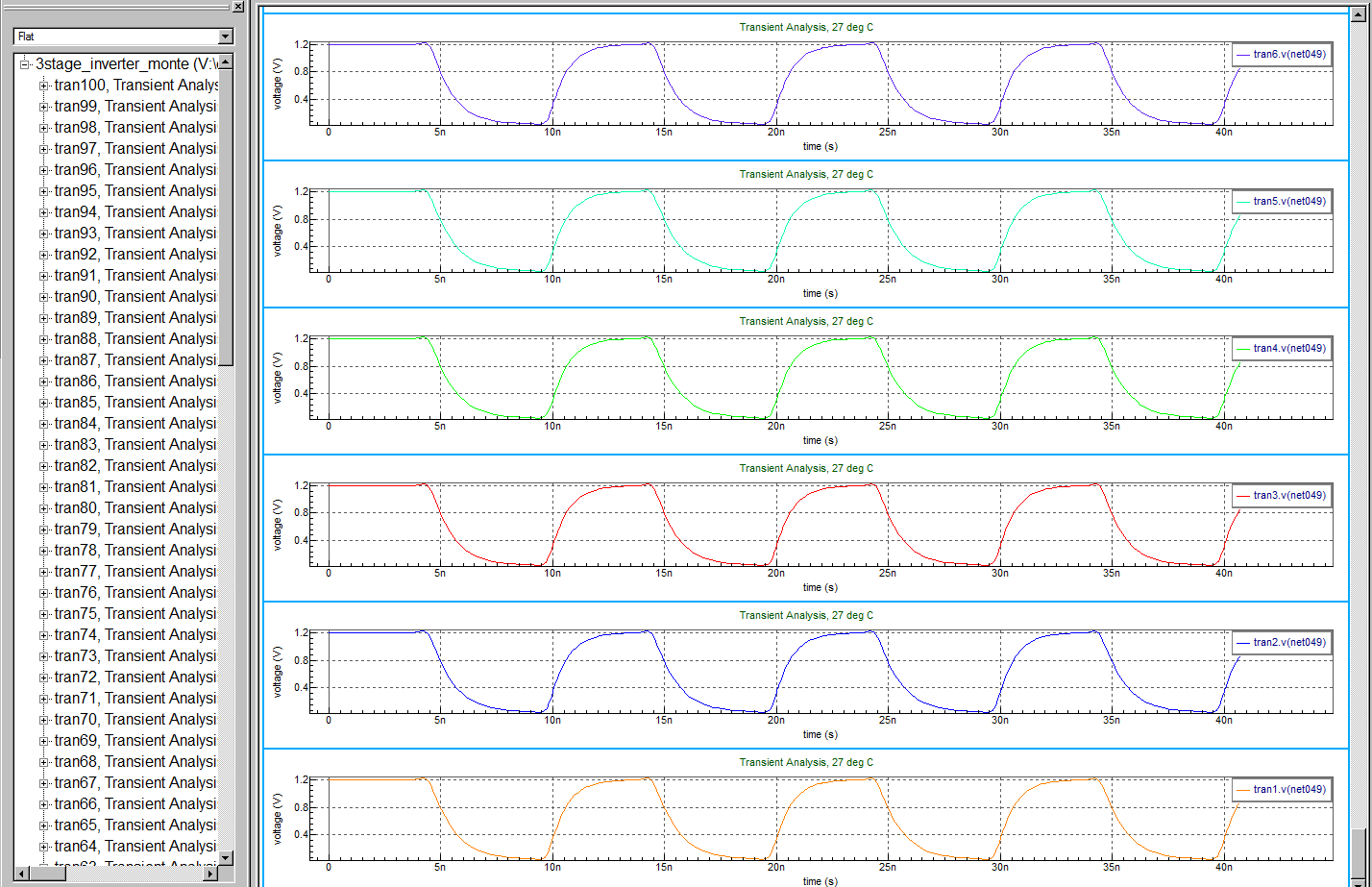
3. In SmartView application create a new cartesian plot window then from SmartSpice plot the Meas – “del_rise” vector. This stops overwriting the existing plot and brings in the measurement data you will use in the Tools – Histogram dialogue. You will get the following picture
. This was just a check on the results and to get data across, you can delete plot.

4. In the SmartView menu go to Tools – Histogram to bring up the dialogue window. Now Drag-and-drop the “del_rise” vector into the Trace box of the Histogram dialogue
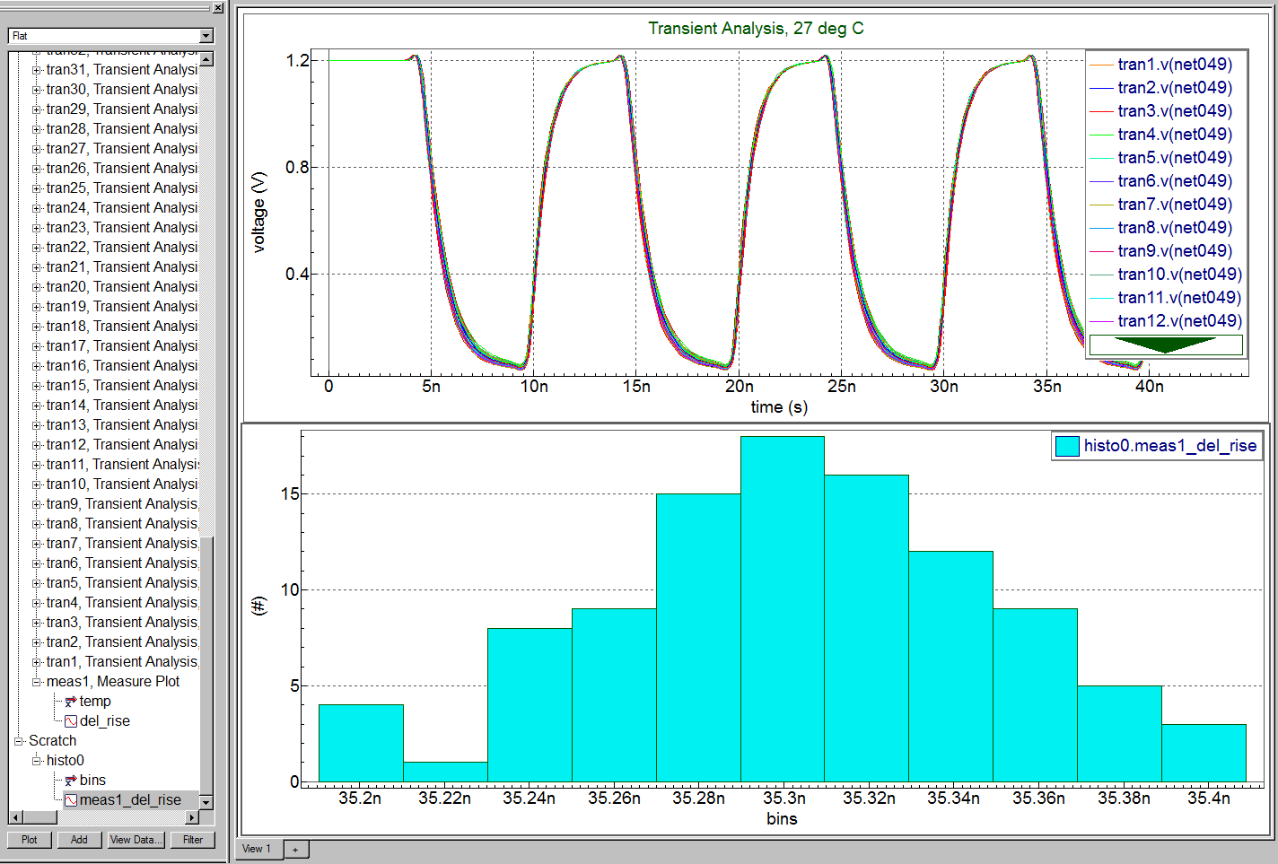
window and press compute to produce Histogram
plot.

The easiest way to check the vectors is in “Vector” window (usually displays in right-bottom corner of the main window) and press the “Plot” button. The second way is to open “Vectors” dialog (View -> Vectors), select required plots in the upper list, and select the required data vectors in the lower list, and press the “Plot” button. The selected vectors will be displayed in SmartView for all the plots selected.

The input deck is a SPICE file containing ……………..

To run the simulation, press the run button. When the simulation completes, the resulting

picture
– Transient set of 100 simulation runs

picture
– Composite set of transient waveforms for (net049)

picture
– Meas plot 1

picture
– Meas plot 2

picture
– Meas plot 3

picture
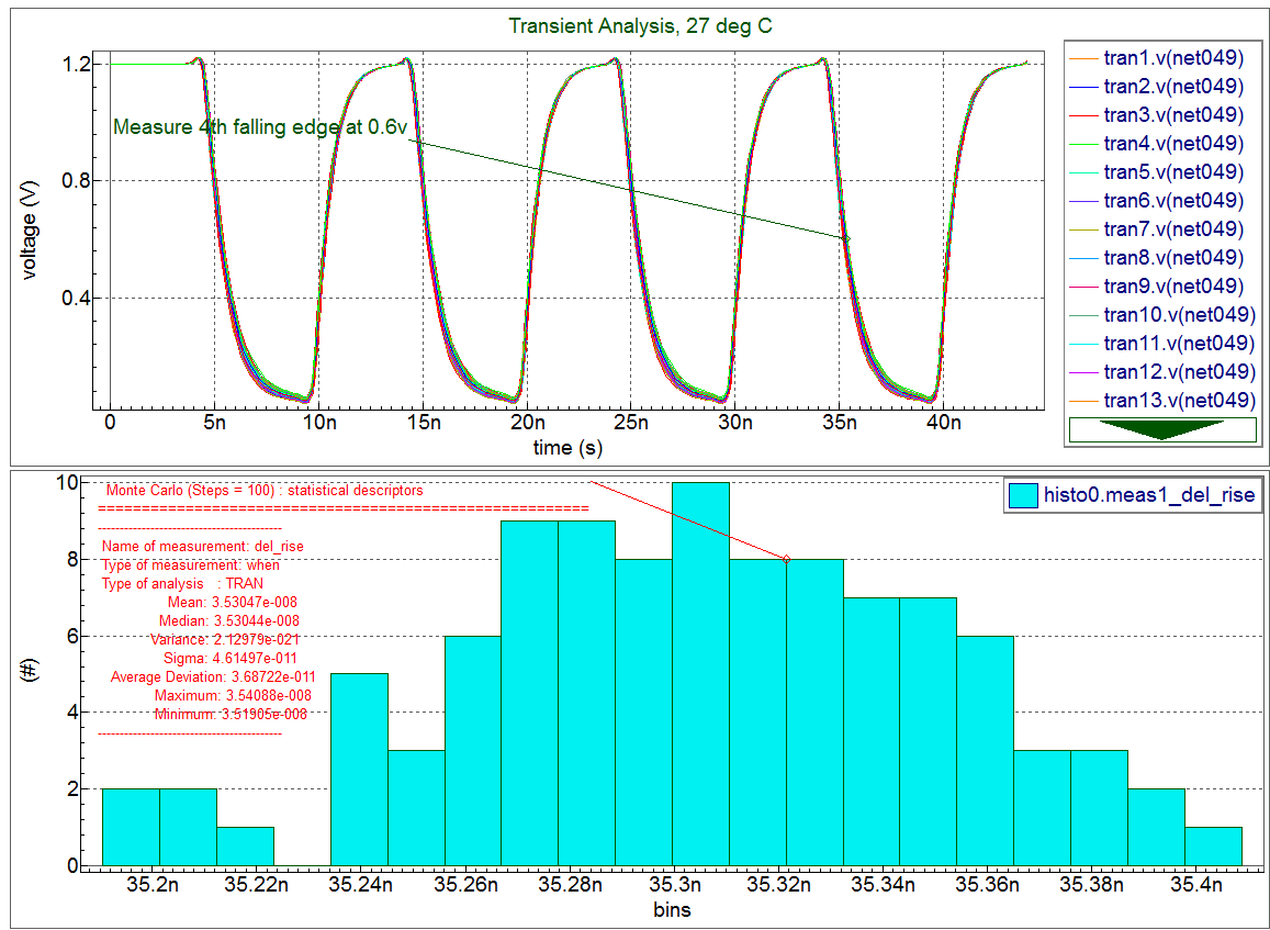
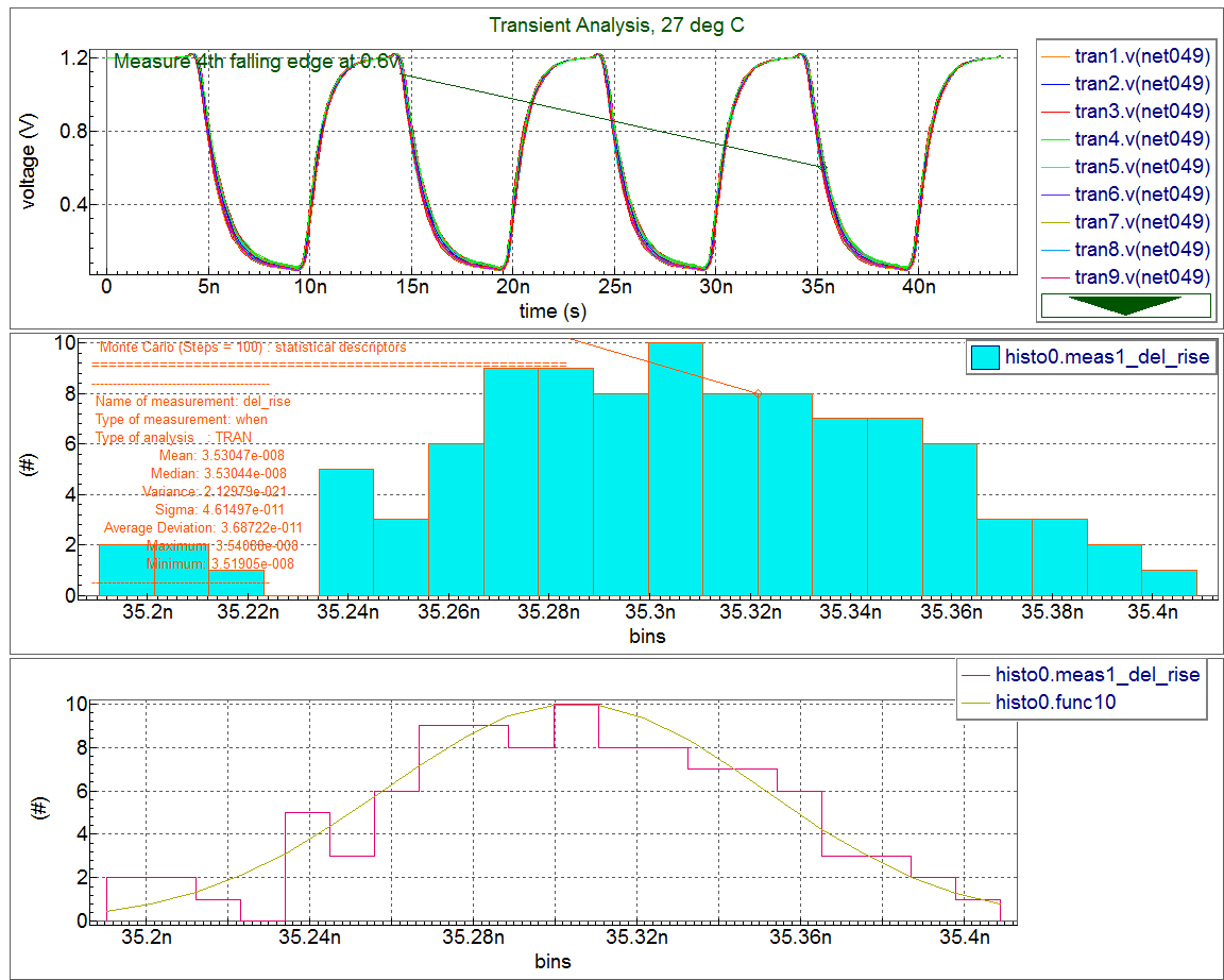
– Basic histogram plot

picture
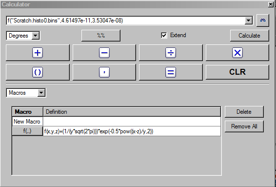
– Calculator equation to use

picture
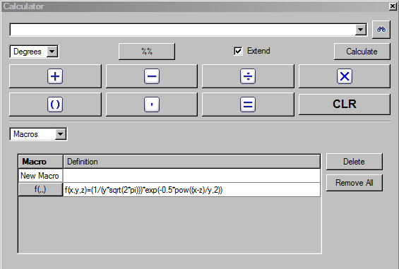
– Use this enetered Macro in calculation

picture
– Show distribution

picture
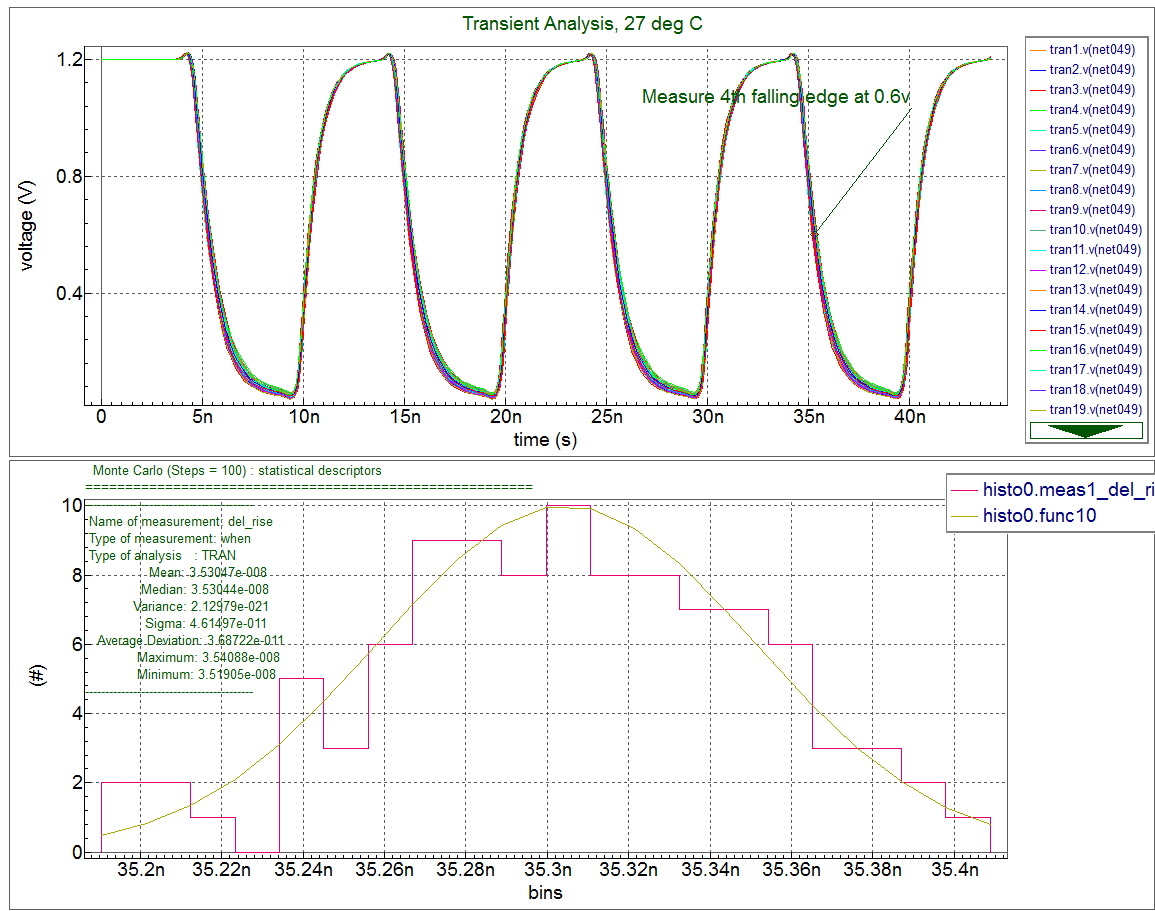
– Final anotated distribution

Graphics

Input Files

3stage_inverter_monte.in

*************************************************
* 3 stage inverter with Monte-Carlo variation   *
*************************************************cs
.param delW= AGAUSS( 0.0, 3u, 3, 1 )
.param clink=10.0e-13  
.param rset=0.5e3

.GLOBAL vcc! 
* File name: test_3stage_inverter_subckt_schematic.s.
XI20 net027 net023 3stage_inverter_block_g2 
V0 net027 0  pulse( 0.0 1.2 2.0e-9 2e-9 2e-9 4e-9 10e-9) 
C0 net049 0  clink M=1.0 
R2 net023 net049  rset M=1.0 
V1 vcc! 0  DC 1.2 

.SUBCKT 3stage_inverter_block_g2 in out 
R7 net12 out  20e-3 M=1.0 
R6 net14 net5  20e-3 M=1.0 
R5 net16 net7  20e-3 M=1.0 
R4 in net9  20e-3 M=1.0 
XI2 net5 net12 Inverter_g1 
XI1 net7 net14 Inverter_g1 
XI0 net9 net16 Inverter_g1 
.ENDS 3stage_inverter_block_g2 

.SUBCKT Inverter_g1 ip_inv op_inv 
R0 net16 op_inv  2e-3 M=1.0 
R1 op_inv net17  2e-3 M=1.0 
M0 net17 ip_inv   0    0   Nch  L=2e-6 W='15e-6 + delW' $*TEMP=100.0 M=1.0 
M1 net16 ip_inv vcc! vcc!  Pch  L=1e-6 W=20e-6          $*TEMP=100.0 M=1.0 
.ENDS Inverter_g1 
*
.option nomod nodeck accurate numdgt=10

.MODEL Nch NMOS level=54 vth0=0.25
.MODEL Pch PMOS level=54 vth0=0.25

.SAVE v(net023) v(net027) v(net049)
**.PRINT TRAN V(net023) V(net027)
.TRAN  0.1n 44.0n sweep monte  100
**.OPTIONS RAWPTS= 100.00 probe   
.TEMP    27.0000 
.MEASURE TRAN DEL_RISE WHEN V(net049)=0.6 FALL=4

.END